Time-dependent toy example

Two illustrative dispatch problems on the same toy database, demonstrating the time-indexed formulation in pulpo.utils.time_extension:

1. One day, hourly resolution — bell-shaped solar peaking at noon, demand with morning and evening peaks. Battery is used for intra-day shifting.

2. Two weeks, daily resolution — variable solar (sunny days, cloudy days, a few breaks in the overcast week) and a weekday/weekend demand pattern. Battery is used for multi-day propagation across the horizon.

Storage logic at a glance

Each storage technology is split into four virtual activities sharing one intermediate product (the charge product):

Activity	Ref. product	Inputs	Role
CHARGE	charge_product	1 kWh electricity	Pumps electricity into storage
HOLD	charge_product	1 unit holdtm1_product	In-step carrier of stored energy
DISCHARGE	electricity, battery	1 unit charge_product	Releases electricity from storage
HOLD t-1	holdtm1_product	— (phantom)	Bridges across timesteps via K

CHARGE and HOLD produce the same product charge_product; PULPO’s choices mechanism unifies them into a single virtual supplier feeding DISCHARGE. The phantom HOLD t-1 produces holdtm1_product; its scaling at \(t\) is locked at 0, but the engine adds a carry-over supply equal to \(K \cdot (\text{charge\_product produced at } t{-}1)\). Because holdtm1_product is a stored product, its time-balance is the inequality

\[ SOC_t \;\le\; K \cdot \bigl(SOC_{t-1} + \text{charged}_{t-1} - \text{discharged}_{t-1}\bigr). \]

The storage spec passed to PULPO is

storage = [(battery_holdtm1, "charge_product", K)]
#          (target_product,    source_product, factor)

K = 1.0 is lossless, K < 1.0 lossy, K = None disables storage.

import bw2data as bd
import matplotlib.pyplot as plt
import numpy as np
import pandas as pd

from pulpo import pulpo_time
from pulpo.datasets.elec_time_database import (
    setup_elec_time_db,
    PROJECT_NAME, DB_NAME,
    SOLAR_KEY, COAL_KEY,
    BATTERY_CHARGE_KEY, BATTERY_HOLD_KEY,
    BATTERY_DISCHARGE_KEY, BATTERY_HOLDTM1_KEY,
    CHARGE_PRODUCT_CHOICE,
)

setup_elec_time_db()
bd.projects.set_current(PROJECT_NAME)
db = bd.Database(DB_NAME)

solar     = next(a for a in db if a.key == SOLAR_KEY)
coal      = next(a for a in db if a.key == COAL_KEY)
charge    = next(a for a in db if a.key == BATTERY_CHARGE_KEY)
hold      = next(a for a in db if a.key == BATTERY_HOLD_KEY)
discharge = next(a for a in db if a.key == BATTERY_DISCHARGE_KEY)
holdtm1   = next(a for a in db if a.key == BATTERY_HOLDTM1_KEY)

GWP100 = str(("GWP", "100a"))

[elec_time_toy] project='elec_time_toy_bw25', db='elec_time_toy_db', activities=6, methods=[('GWP', '100a')]

Shared helpers

Both examples reuse the same scenario solver and dispatch plot. Each scenario is parameterised by K (round-trip retention factor) and the per-step input dictionaries.

def build_inputs(time_steps, solar_cap, demand_kwh):
    """Assemble (choices, demand, upper_limit, lower_limit) for the toy DB."""
    choices = {
        "electricity":         {solar: float('inf'), coal: float('inf'), discharge: float('inf')},
        CHARGE_PRODUCT_CHOICE: {charge: float('inf'), hold: float('inf')},
    }
    upper_limit = {
        t: {
            solar: solar_cap[t],
            coal: float('inf'),
            charge: float('inf'),
            hold: float('inf'),
            # battery starts empty -> nothing to discharge at t=0
            discharge: 0.0 if t == time_steps[0] else float('inf'),
            holdtm1: 0.0,  # phantom
        }
        for t in time_steps
    }
    # battery flows must be non-negative (default lower bound is -inf)
    lower_limit = {t: {charge: 0.0, hold: 0.0, discharge: 0.0} for t in time_steps}
    demand = {t: {"electricity": demand_kwh[t]} for t in time_steps}
    return choices, demand, upper_limit, lower_limit


def solve_scenario(label, *, K, time_steps, step_labels,
                   solar_cap, demand_kwh):
    choices, demand, upper_limit, lower_limit = build_inputs(
        time_steps, solar_cap, demand_kwh)
    storage_spec = [(holdtm1, CHARGE_PRODUCT_CHOICE, K)] if K is not None else None
    w = pulpo_time.PulpoOptimizerTime(PROJECT_NAME, DB_NAME, {GWP100: 1})
    w.get_lci_data()
    w.instantiate(
        choices=choices, demand=demand,
        upper_limit=upper_limit, lower_limit=lower_limit,
        time_steps=time_steps, storage=storage_spec,
    )
    w.solve()
    pmap = w.lci_data["process_map"]
    df = pd.DataFrame(
        {name: [w.instance.scaling_vector[t, pmap[a.key]].value for t in time_steps]
         for name, a in [("solar", solar), ("coal", coal),
                         ("charge", charge), ("hold", hold),
                         ("discharge", discharge)]},
        index=step_labels,
    )
    df["co2"] = [w.instance.impacts[t, GWP100].value for t in time_steps]
    df.attrs.update(label=label, K=K, total_co2=float(df["co2"].sum()))
    return df


def stored_energy_series(df, K):
    """SOC entering each step: SOC_t = K*(SOC_{t-1} + charge_{t-1} - discharge_{t-1})."""
    if K is None:
        return [0.0] * len(df)
    soc = [0.0]
    for t in range(len(df) - 1):
        soc.append(K * (soc[-1] + df["charge"].iloc[t] - df["discharge"].iloc[t]))
    return soc


def plot_dispatch(dfs, time_steps, step_labels, demand_kwh,
                  separators=(), title=""):
    x = np.arange(len(time_steps))
    fig, axes = plt.subplots(len(dfs), 1, figsize=(11, 3.0 * len(dfs)),
                             sharex=True)
    if len(dfs) == 1:
        axes = [axes]
    for ax, df in zip(axes, dfs):
        bottoms = np.zeros(len(time_steps))
        for col, color, lab in [("solar",     "#f4a826", "solar"),
                                ("discharge", "#9b59b6", "discharge (out)"),
                                ("coal",      "#5d5d5d", "coal")]:
            v = df[col].values
            ax.bar(x, v, bottom=bottoms, label=lab, color=color, edgecolor="white")
            bottoms = bottoms + v
        ax.bar(x, -df["charge"].values, color="none", edgecolor="#2ca02c",
               hatch="//", linewidth=1.0, label="charge (into battery)")
        if df.attrs["K"] is not None:
            ax2 = ax.twinx()
            ax2.plot(x, stored_energy_series(df, df.attrs["K"]),
                     "o--", color="#2ca02c", markersize=4,
                     label="state of charge")
            ax2.set_ylabel("SOC [kWh]", color="#2ca02c")
            ax2.tick_params(axis='y', labelcolor="#2ca02c")
        ax.plot(x, [demand_kwh[t] for t in time_steps], "k_", markersize=10,
                markeredgewidth=2, label="demand")
        for s in separators:
            ax.axvline(s, color="k", linestyle=":", linewidth=1)
        ax.axhline(0, color="black", linewidth=0.6)
        ax.set_title(f"{df.attrs['label']}  -  CO2 = {df.attrs['total_co2']:.1f} kg")
        ax.grid(axis="y", alpha=0.3)
        ax.set_ylabel("kWh\n(- charge | + supply +)")
    axes[-1].set_xticks(x)
    axes[-1].set_xticklabels(step_labels, rotation=45, ha="right")
    axes[0].legend(loc="upper right", fontsize=8, ncol=2)
    if title:
        fig.suptitle(title)
    fig.tight_layout(); plt.show()

Example 1 — One day, hourly resolution

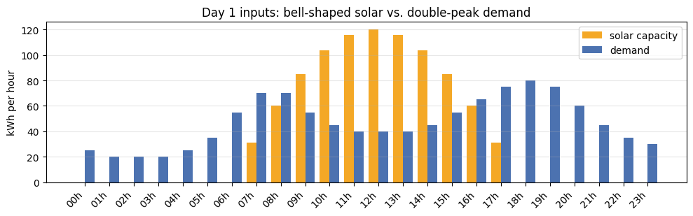
24 hourly steps. Solar follows a bell curve peaking at 120 kWh at noon (zero before sunrise and after sunset). Demand has the classic double-peak shape: quiet at night, a morning ramp, a midday plateau, and a strong evening peak.

The storage role here is short-term: charge midday surplus to cover the evening peak.

# 24 hourly steps; bell-shaped solar, double-peak demand
time_steps_h  = list(range(24))
step_labels_h = [f"{t:02d}h" for t in time_steps_h]

solar_cap_h  = {t: v for t, v in enumerate([0.0, 0.0, 0.0, 0.0, 0.0, 0.0, 0.0, 31.1, 60.0, 84.9, 103.9, 115.9, 120.0, 115.9, 103.9, 84.9, 60.0, 31.1, 0.0, 0.0, 0.0, 0.0, 0.0, 0.0])}
demand_kwh_h = {t: v for t, v in enumerate([25, 20, 20, 20, 25, 35, 55, 70, 70, 55, 45, 40, 40, 40, 45, 55, 65, 75, 80, 75, 60, 45, 35, 30])}

x = np.arange(24)
width = 0.4
fig, ax = plt.subplots(figsize=(10, 3.2))
ax.bar(x - width/2, [solar_cap_h[t]  for t in time_steps_h], width,
       label="solar capacity", color="#f4a826")
ax.bar(x + width/2, [demand_kwh_h[t] for t in time_steps_h], width,
       label="demand",          color="#4c72b0")
ax.set_xticks(x); ax.set_xticklabels(step_labels_h, rotation=45, ha="right")
ax.set_ylabel("kWh per hour")
ax.set_title("Day 1 inputs: bell-shaped solar vs. double-peak demand")
ax.legend(loc="upper right"); ax.grid(axis="y", alpha=0.3)
fig.tight_layout(); plt.show()

kwargs_h = dict(time_steps=time_steps_h, step_labels=step_labels_h,
                solar_cap=solar_cap_h, demand_kwh=demand_kwh_h)
df_h_none  = solve_scenario("no battery",            K=None, **kwargs_h)
df_h_lossy = solve_scenario("battery (K = 0.95)",    K=0.95, **kwargs_h)
df_h_ideal = solve_scenario("~ideal battery (K=0.999)", K=0.999, **kwargs_h)

for df in (df_h_none, df_h_lossy, df_h_ideal):
    print(f"  {df.attrs['label']:25s}  total CO2 = {df.attrs['total_co2']:7.2f} kg")

Creating time-indexed instance
Time-indexed instance created
optimal solution found:  622.8
Optimization problem solved using Highspy
Creating time-indexed instance
Time-indexed instance created
optimal solution found:  332.8151255356928
Optimization problem solved using Highspy
Creating time-indexed instance
Time-indexed instance created
optimal solution found:  248.9
Optimization problem solved using Highspy
  no battery                 total CO2 =  622.80 kg
  battery (K = 0.95)         total CO2 =  332.82 kg
  ~ideal battery (K=0.999)   total CO2 =  248.90 kg

plot_dispatch([df_h_none, df_h_lossy, df_h_ideal],
              time_steps_h, step_labels_h, demand_kwh_h,
              title="Intra-day dispatch (24 hourly steps)")

Discussion — what the optimizer is doing

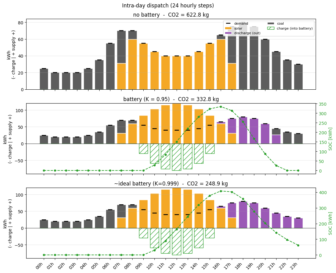
• No battery (622.8 kg). Solar alone covers the midday plateau. The morning ramp, the entire night, and especially the strong evening peak (16h–22h) are served by coal — the bulk of the emissions sit in the evening hours when there is no sun left.

• Lossy battery, K = 0.95 (332.8 kg). The optimizer stores the whole solar surplus of 09h–15h and discharges it from 16h on. Every hour held costs 5 %, so the stored energy runs out at 21h and coal serves the last hours of the evening.

• Nearly ideal battery, K = 0.999 (248.9 kg). Same intra-day shape, but the stored surplus now lasts until midnight. The night and the morning before sunrise still run on coal: the battery starts the day empty.

Why K = 0.999 and not 1.0? With a lossless battery, running 1 kWh of coal at 03h, charging it and discharging it at 06h emits exactly as much CO₂ as running that coal at 06h. The LP then has many equally good dispatches, and a solver may return one with pointless charge/discharge cycles. A tiny loss makes every round trip cost something and singles out the dispatch without them.

Example 2 — Two weeks, daily resolution

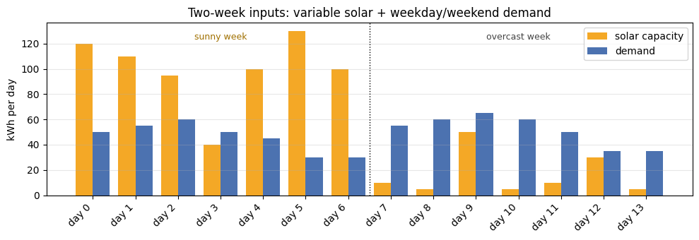
14 daily steps. Solar mostly follows a sunny / overcast pattern with realistic variability: a partly cloudy day in week 1 and two short sunny breaks in week 2. Demand drops on weekends (days 5–6 and 12–13).

The storage role here is multi-step propagation: the optimizer must transport week-1 surplus across many days to cover week-2 demand — feasible only because HOLD recycles charge_product from one step to the next, paying a factor of K each time.

# 14 daily steps; varied solar + weekday/weekend demand
time_steps_d  = list(range(14))
step_labels_d = [f"day {t}" for t in time_steps_d]

solar_cap_d  = {t: v for t, v in enumerate([120, 110, 95, 40, 100, 130, 100, 10, 5, 50, 5, 10, 30, 5])}
demand_kwh_d = {t: v for t, v in enumerate([50, 55, 60, 50, 45, 30, 30, 55, 60, 65, 60, 50, 35, 35])}

x = np.arange(14)
width = 0.4
fig, ax = plt.subplots(figsize=(10, 3.5))
ax.bar(x - width/2, [solar_cap_d[t]  for t in time_steps_d], width,
       label="solar capacity", color="#f4a826")
ax.bar(x + width/2, [demand_kwh_d[t] for t in time_steps_d], width,
       label="demand",          color="#4c72b0")
ax.axvline(6.5, color="k", linestyle=":", linewidth=1)
ymax = max(max(solar_cap_d.values()), max(demand_kwh_d.values()))
ax.text(3.0,  ymax * 0.95, "sunny week",    ha="center", fontsize=9, color="#a07000")
ax.text(10.0, ymax * 0.95, "overcast week", ha="center", fontsize=9, color="#444")
ax.set_xticks(x); ax.set_xticklabels(step_labels_d, rotation=45, ha="right")
ax.set_ylabel("kWh per day")
ax.set_title("Two-week inputs: variable solar + weekday/weekend demand")
ax.legend(loc="upper right"); ax.grid(axis="y", alpha=0.3)
fig.tight_layout(); plt.show()

kwargs_d = dict(time_steps=time_steps_d, step_labels=step_labels_d,
                solar_cap=solar_cap_d, demand_kwh=demand_kwh_d)
df_d_none  = solve_scenario("no battery",             K=None, **kwargs_d)
df_d_lossy = solve_scenario("battery (K = 0.85)",     K=0.85, **kwargs_d)
df_d_ideal = solve_scenario("~ideal battery (K = 0.999)",K=0.999, **kwargs_d)

for df in (df_d_none, df_d_lossy, df_d_ideal):
    print(f"  {df.attrs['label']:30s}  total CO2 = {df.attrs['total_co2']:7.2f} kg")

Creating time-indexed instance
Time-indexed instance created
optimal solution found:  255.0
Optimization problem solved using Highspy
Creating time-indexed instance
Time-indexed instance created
optimal solution found:  75.61739504764356
Optimization problem solved using Highspy
Creating time-indexed instance
Time-indexed instance created
optimal solution found:  0.0
Optimization problem solved using Highspy
  no battery                      total CO2 =  255.00 kg
  battery (K = 0.85)              total CO2 =   75.62 kg
  ~ideal battery (K = 0.999)      total CO2 =    0.00 kg

plot_dispatch([df_d_none, df_d_lossy, df_d_ideal],
              time_steps_d, step_labels_d, demand_kwh_d,
              separators=(6.5,),
              title="Two-week dispatch (14 daily steps)")

Discussion — what the optimizer is doing

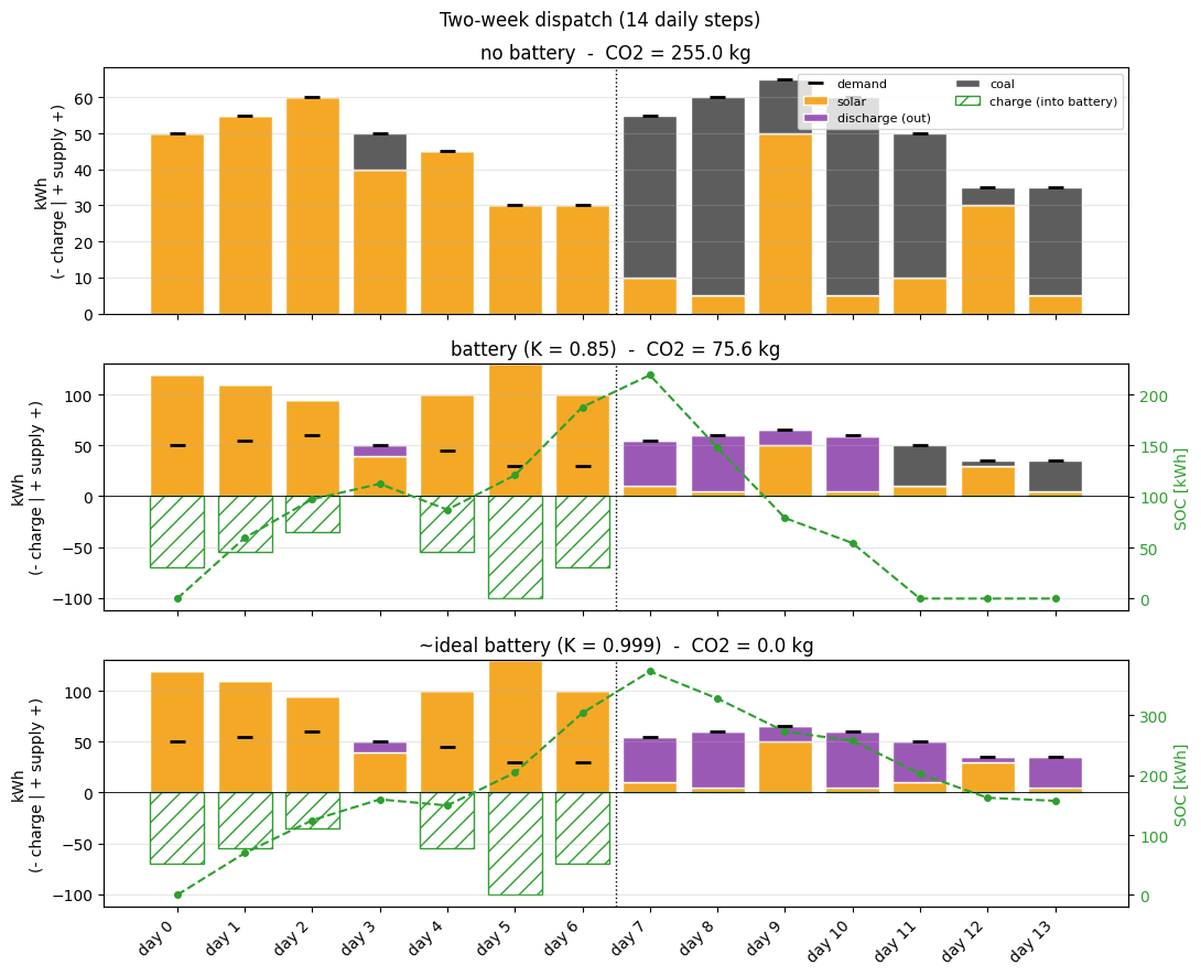
• No battery (255.0 kg). Week-1 sunny days (mostly 100–130 kWh of solar) cover their own demand and waste the surplus; the cloudy day (day 3, 40 kWh) and almost the whole of week 2 must be filled by coal. The two short sunny breaks in week 2 (day 9, day 12) only nibble at the deficit.

• Lossy battery, K = 0.85 (75.6 kg). The optimizer stores the surplus of every sunny week-1 day (day 0–2, day 4–6) and spends it on the cloudy day 3 and in week 2. Week 2 has nothing to store: even its sunny breaks stay below demand. Every day held costs 15 % (energy carried from day 6 to day 10 keeps \(0.85^{4} \approx 52\,\%\)), so the stored energy is used up on day 10 and coal covers day 11–13.

• Nearly ideal battery, K = 0.999 (0.0 kg). The week-1 surplus alone covers all of week-2 demand, so coal is fully eliminated. The state of charge climbs through week 1 (with a dip on the cloudy day 3) and decays through week 2, the textbook seasonal-storage shape.

The contrast between the two K values shows the value of the HOLD activity explicitly: it is the only mechanism that lets charge_product propagate across non-adjacent timesteps, and the K factor turns each step held into a real economic cost (otherwise the optimizer would be indifferent to when it charges).